library(sfdep)
library(dplyr)

geoms <- guerry$geometry
centroids <- sf::st_centroid(geoms)

nb <- st_contiguity(geoms)
wt <- st_kernel_weights(nb, centroids, "gaussian")Encoding spatial patterns as variables
Principal Coordinate Analysis & Moran Eigenvectors
spatial
r
I’ve begun reading “Spatial modelling: a comprehensive framework for principal coordinate analysis of neighbour matrices (PCNM)” which describes the process of making “Moran Eigenvector Maps.”
In this case, I haven’t finished reading the paper but am quite thrilled by the prospect of it. One of the biggest problems in ecological and social science modelling is that space is often a confounder in models. By this I mean that a lot of phenomena we see are spatially dependent.
Reductively, spatial dependence means that variables or outcomes are strongly linked to where things are. For example, income tends to be spatially dependent. Meaning that high income areas are typically surounded by other high income areas.
The problem
When modelling data that exhibit spatial dependence, spatial relationships need to be accounted for. Otherwise, you will often find that model residuals (errors) also exhibit spatial dependence. So? How can you control for this.
There are a number of techniques that people use from more statistically sound ones, to tricks used by ML engineers. For example you may introduce the spatial lag (neighborhood average of a variable) to account for some of the spatial association.
Principal Coordinate Analysis (PCoA)
One interesting idea is using principle components analysis to encode geography into numeric variables. Conceptually, the idea is actually rather simple!
When we do spatial statistics, we create what are called spatial weights matrices. These define which features are related to eachother.
For example we can identify the neighbors from the famous guerry dataset based on the contiguity—that is if they are touching. We create a nb and wt object. The nb are the neighbors and wt uses a gaussian kernel. The gaussian kernel assigns more weight to to locations that are closer and less weight to those that are further—essentially following the normal distribution.
Visually, this is what the neighborhood relationship looks like:
Code
library(ggplot2)
sfn <- st_as_graph(geoms, nb, )

autoplot(sfn) +
  geom_sf(data = geoms, fill = NA, color = "black", lwd = 0.2) +
  theme_void()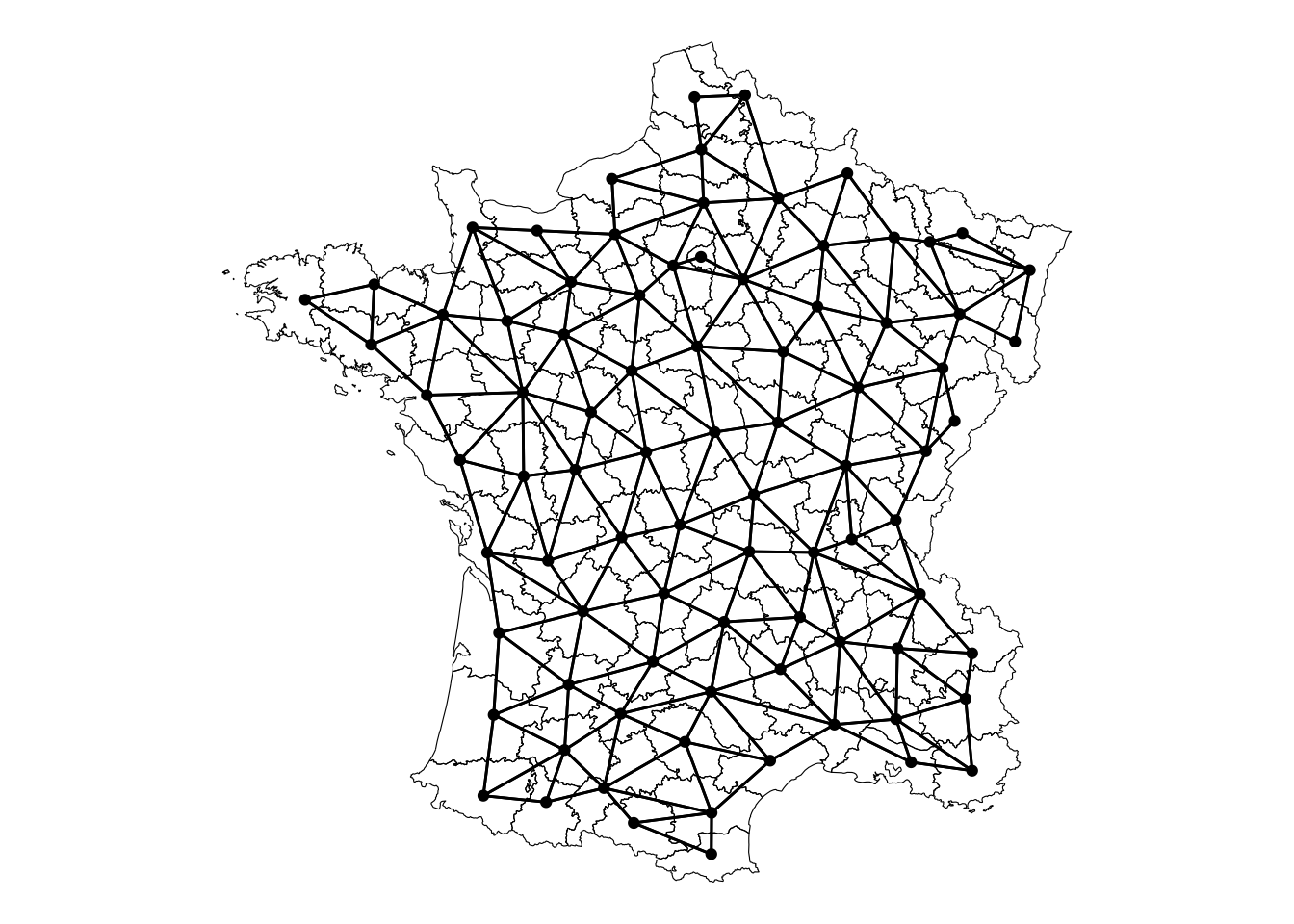
The weights object is a ragged array which is used to be a sparse matrix representation of the spatial weights.
head(wt)[[1]]
[1] 1.553402 1.857660 2.062100 1.676694
[[2]]
[1] 1.801787 1.717777 1.439955 1.721547 1.260566 1.429496
[[3]]
[1] 1.599532 1.527097 1.376795 1.722723 1.865664 1.350771
[[4]]
[1] 2.040754 1.356645 1.871658 1.685343
[[5]]
[1] 2.040754 1.674375 1.689488
[[6]]
[1] 2.075805 1.679763 1.357435 1.308397 2.009760 1.812262 1.432539The spatial weights are an n x n square matrix. The idea behind the paper above is that we can encode the spatial relationships in this neighborhood matrix using principle components.
We can take the weights matrix and create a dense matrix from it:
m <- wt_as_matrix(nb, wt)Using this new matrix, we can perform PCA on it.
Importance of components:
                           PC1     PC2     PC3     PC4     PC5     PC6     PC7
Standard deviation     0.95957 0.89585 0.85836 0.81484 0.79239 0.72065 0.66135
Proportion of Variance 0.06928 0.06038 0.05543 0.04996 0.04724 0.03907 0.03291
Cumulative Proportion  0.06928 0.12966 0.18510 0.23505 0.28229 0.32137 0.35428
                           PC8     PC9    PC10    PC11    PC12    PC13    PC14
Standard deviation     0.65347 0.60391 0.58993 0.54551 0.51607 0.51048 0.50266
Proportion of Variance 0.03213 0.02744 0.02618 0.02239 0.02004 0.01961 0.01901
Cumulative Proportion  0.38640 0.41385 0.44003 0.46242 0.48246 0.50206 0.52107
                          PC15    PC16    PC17    PC18    PC19    PC20    PC21
Standard deviation     0.50008 0.49651 0.48004 0.47334 0.46571 0.46447 0.45886
Proportion of Variance 0.01882 0.01855 0.01734 0.01686 0.01632 0.01623 0.01584
Cumulative Proportion  0.53989 0.55844 0.57578 0.59263 0.60895 0.62518 0.64103
                          PC22   PC23    PC24    PC25    PC26    PC27    PC28
Standard deviation     0.45371 0.4495 0.43495 0.43208 0.42533 0.42265 0.40912
Proportion of Variance 0.01549 0.0152 0.01423 0.01405 0.01361 0.01344 0.01259
Cumulative Proportion  0.65651 0.6717 0.68595 0.70000 0.71361 0.72705 0.73964
                          PC29    PC30    PC31    PC32    PC33    PC34    PC35
Standard deviation     0.40662 0.40248 0.39657 0.38949 0.38172 0.37648 0.36612
Proportion of Variance 0.01244 0.01219 0.01183 0.01141 0.01096 0.01066 0.01009
Cumulative Proportion  0.75208 0.76427 0.77610 0.78752 0.79848 0.80915 0.81923
                          PC36    PC37    PC38    PC39    PC40    PC41    PC42
Standard deviation     0.35885 0.35324 0.35042 0.34655 0.33906 0.33458 0.32477
Proportion of Variance 0.00969 0.00939 0.00924 0.00904 0.00865 0.00842 0.00794
Cumulative Proportion  0.82892 0.83831 0.84755 0.85658 0.86523 0.87366 0.88159
                          PC43    PC44    PC45    PC46    PC47    PC48    PC49
Standard deviation     0.32182 0.30859 0.30426 0.30100 0.29700 0.28072 0.27493
Proportion of Variance 0.00779 0.00716 0.00697 0.00682 0.00664 0.00593 0.00569
Cumulative Proportion  0.88938 0.89655 0.90351 0.91033 0.91697 0.92290 0.92858
                          PC50    PC51    PC52    PC53    PC54    PC55    PC56
Standard deviation     0.26620 0.25927 0.25817 0.25373 0.25203 0.23148 0.22505
Proportion of Variance 0.00533 0.00506 0.00501 0.00484 0.00478 0.00403 0.00381
Cumulative Proportion  0.93391 0.93897 0.94399 0.94883 0.95361 0.95764 0.96145
                          PC57   PC58    PC59    PC60    PC61    PC62    PC63
Standard deviation     0.21925 0.2124 0.20738 0.20542 0.20426 0.17969 0.17415
Proportion of Variance 0.00362 0.0034 0.00324 0.00318 0.00314 0.00243 0.00228
Cumulative Proportion  0.96507 0.9685 0.97170 0.97488 0.97801 0.98044 0.98273
                          PC64    PC65    PC66    PC67    PC68    PC69    PC70
Standard deviation     0.17330 0.16078 0.15374 0.14641 0.14201 0.13335 0.13088
Proportion of Variance 0.00226 0.00194 0.00178 0.00161 0.00152 0.00134 0.00129
Cumulative Proportion  0.98499 0.98693 0.98871 0.99032 0.99184 0.99318 0.99447
                          PC71    PC72    PC73    PC74    PC75    PC76    PC77
Standard deviation     0.12526 0.10810 0.10181 0.08943 0.08425 0.07410 0.07172
Proportion of Variance 0.00118 0.00088 0.00078 0.00060 0.00053 0.00041 0.00039
Cumulative Proportion  0.99565 0.99653 0.99731 0.99791 0.99844 0.99885 0.99924
                          PC78    PC79    PC80    PC81    PC82    PC83     PC84
Standard deviation     0.06809 0.04608 0.03760 0.03481 0.02250 0.01105 0.008143
Proportion of Variance 0.00035 0.00016 0.00011 0.00009 0.00004 0.00001 0.000000
Cumulative Proportion  0.99959 0.99975 0.99986 0.99995 0.99999 1.00000 1.000000
                            PC85
Standard deviation     3.921e-16
Proportion of Variance 0.000e+00
Cumulative Proportion  1.000e+00
The spatial relationships that are embedded by the spatial weights matrix, are now encoded as components from a PCA. This means that we can use each of these components as a univariate measure of space. And, they also exhibit quite interesting patterns of spatial dependence.
Exploring PCoA
These components essentially capture spatial autocorrelation. For example we an look at the first component.
# extract the first component
comp1 <- pca_res$rotation[, 1]

ggplot(guerry, aes(fill = comp1)) +
  geom_sf(color = "black", lwd = 0.2) +
  scale_fill_viridis_c() +
  theme_void() +
  labs(fill = "Eigenvector")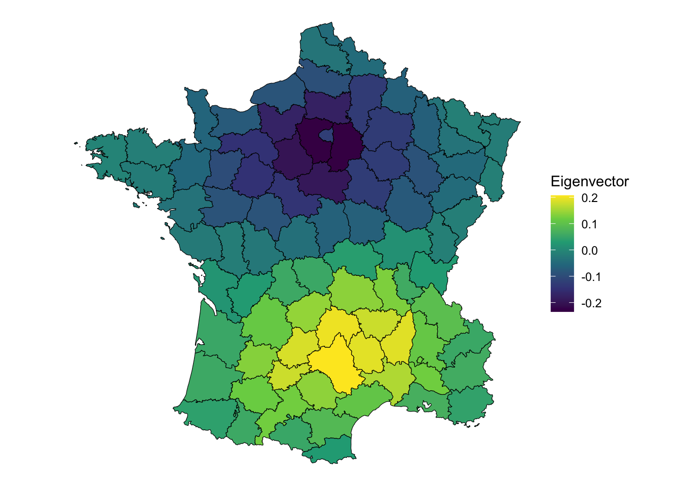
It displays a pattern of being near Paris (the dark purple, or negative eigenvector values) or being nearer to Aveyron, the positive eigenvector values. Clearly, this displays some interesting global spatial autocorrelation. But how much?
We can measure the global spatial autocorrelation of this component using Moran’s I.
global_moran_perm(comp1, nb, wt)
    Monte-Carlo simulation of Moran I

data:  x
weights: listw
number of simulations + 1: 500

statistic = 1.0698, observed rank = 500, p-value < 2.2e-16
alternative hypothesis: two.sided
The result is 1.0698 which is greater than the theoretical maximum of 1. There is a ridiculous amount of spatial autocorrelation here.
Using PCoA Eigenvectors to reduce spatial confounding
Predicting crime based on population and the prostitution levels of 1830s France shows that there is a lot of spatial autocorrelation in the residuals. This means that the results of the model do not appropriately account for spatial dependence.
Call:
lm(formula = crime_pers ~ pop1831 + prostitutes, data = guerry)

Residuals:
     Min       1Q   Median       3Q      Max
-13762.2  -4592.1   -974.6   4892.4  18672.5

Coefficients:
             Estimate Std. Error t value Pr(>|t|)
(Intercept) 13688.932   2265.393   6.043 4.27e-08 ***
pop1831        17.676      5.881   3.006  0.00352 **
prostitutes    -3.197      1.665  -1.920  0.05833 .
---
Signif. codes:  0 '***' 0.001 '**' 0.01 '*' 0.05 '.' 0.1 ' ' 1

Residual standard error: 7001 on 82 degrees of freedom
Multiple R-squared:  0.1021,    Adjusted R-squared:  0.08016
F-statistic: 4.66 on 2 and 82 DF, p-value: 0.01211global_moran_test(resid(mod), nb, wt)
    Moran I test under randomisation

data:  x
weights: listw

Moran I statistic standard deviate = 5.0424, p-value = 2.298e-07
alternative hypothesis: greater
sample estimates:
Moran I statistic       Expectation          Variance
      0.328493924      -0.011904762       0.004557168
If you include the first eigenvector component, the spatial autocorrelation of the residuals decrease dramatically.
Call:
lm(formula = crime_pers ~ pop1831 + prostitutes + comp1, data = guerry)

Residuals:
     Min       1Q   Median       3Q      Max
-14228.8  -3822.7   -893.4   4232.5  19718.8

Coefficients:
              Estimate Std. Error t value Pr(>|t|)
(Intercept)  14847.292   2080.269   7.137 3.66e-10 ***
pop1831         15.179      5.386   2.818  0.00607 **
prostitutes     -4.597      1.551  -2.964  0.00399 **
comp1       -28422.828   6708.123  -4.237 5.95e-05 ***
---
Signif. codes:  0 '***' 0.001 '**' 0.01 '*' 0.05 '.' 0.1 ' ' 1

Residual standard error: 6373 on 81 degrees of freedom
Multiple R-squared:  0.265, Adjusted R-squared:  0.2378
F-statistic: 9.733 on 3 and 81 DF, p-value: 1.482e-05global_moran_test(resid(mod), nb, wt)
    Moran I test under randomisation

data:  x
weights: listw

Moran I statistic standard deviate = 2.666, p-value = 0.003838
alternative hypothesis: greater
sample estimates:
Moran I statistic       Expectation          Variance
      0.167439656      -0.011904762       0.004525529
Interestingly, this increases the prostitutes variable increases and the
What about another component?
We can plot the relationship that is capture by the second component.
# extract the second component
comp2 <- pca_res$rotation[, 2]

ggplot(guerry, aes(fill = comp2)) +
  geom_sf(color = "black", lwd = 0.2) +
  scale_fill_viridis_c() +
  theme_void() +
  labs(fill = "Eigenvector")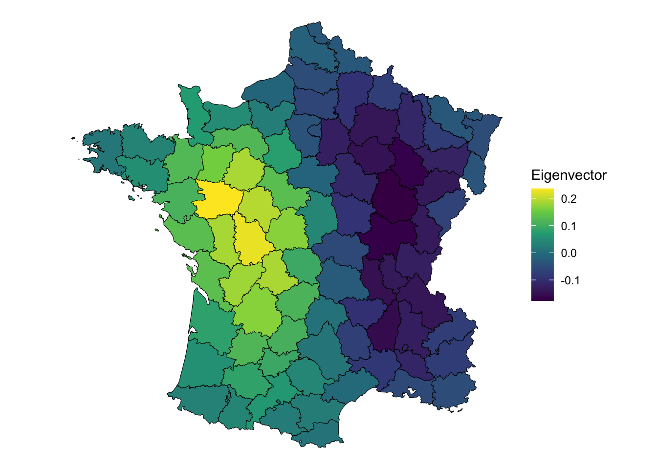
This component captures a west to east relationship rather than a north to south one. Is the second component spatially autocorrelated?
global_moran_perm(comp2, nb, wt)
    Monte-Carlo simulation of Moran I

data:  x
weights: listw
number of simulations + 1: 500

statistic = 0.99864, observed rank = 500, p-value < 2.2e-16
alternative hypothesis: two.sided
Oh hell yeah it is.
If this component is included in the model instead of the first one we see something interesting.
Call:
lm(formula = crime_pers ~ pop1831 + prostitutes + comp2, data = guerry)

Residuals:
   Min     1Q Median     3Q    Max
-13617  -4584  -1150   4831  18360

Coefficients:
             Estimate Std. Error t value Pr(>|t|)
(Intercept) 13730.388   2278.027   6.027 4.71e-08 ***
pop1831        17.518      5.919   2.960  0.00404 **
prostitutes    -3.098      1.686  -1.837  0.06989 .
comp2        3303.053   7091.459   0.466  0.64262
---
Signif. codes:  0 '***' 0.001 '**' 0.01 '*' 0.05 '.' 0.1 ' ' 1

Residual standard error: 7034 on 81 degrees of freedom
Multiple R-squared:  0.1045,    Adjusted R-squared:  0.0713
F-statistic: 3.15 on 3 and 81 DF, p-value: 0.02941global_moran_test(resid(mod), nb, wt)
    Moran I test under randomisation

data:  x
weights: listw

Moran I statistic standard deviate = 5.0189, p-value = 2.598e-07
alternative hypothesis: greater
sample estimates:
Moran I statistic       Expectation          Variance
      0.326953780      -0.011904762       0.004558477
The model is not impacted nor is the spatial autocorrelation. So the pattern encompassed by the second component is not confounding our variables like the first one is.
What does this mean?
If you have spatially dependent features that you’re predicting you should consider using these as input features to your models. I have a hunch that they would work insanely well with computer vision tasks and things models like Random Forests and XGBoost.