trendyy is a package for querying Google Trends. It is build around Philippe Massicotte’s package gtrendsR which accesses this data wonderfully.
The inspiration for this package was to provide a tidy interface to the trends data.
Getting Started
Installation
You can install trendyy from CRAN using install.packages("trendyy").
Usage
Use trendy() to search Google Trends. The only mandatory argument is search_terms. This is a character vector with the terms of interest. It is important to note that Google Trends is only capable of comparing up to five terms. Thus, if your search_terms vector is longer than 5, it will search each term individually. This will remove the direct comparative advantage that Google Trends gives you.
Additional arguments

from: The beginning date of the query in"YYYY-MM-DD"format.to: The end date of the query in"YYYY-MM-DD"format....: any additional arguments that would be passed togtrendsR::gtrends(). Note that it might be useful to indicate the geography of interest. SeegtrendsR::countriesfor list of possible geographies.
Accessor Functions
get_interest(): Retrieve interest over timeget_interest_city(): Retrieve interest by cityget_interest_country(): Retrieve interest by countryget_interest_dma(): Retrieve interest by DMAget_interest_region(): Retrieve interest by regionget_related_queries(): Retrieve related queriesget_related_topics(): Retrieve related topics
Example
Seeing as I found an interest in this due to the relatively pervasive use of Google Trends in political analysis, I will compare the top five polling candidates in the 2020 Democratic Primary. As of May 22nd, they were Joe Biden, Kamala Harris, Beto O’Rourke, Bernie Sanders, and Elizabeth Warren.
First, I will create a vector of my desired search terms. Second, I will pass that vector to trendy() specifying my query date range from the first of 2019 until today (May 25th, 2019).
candidates <- c("Joe Biden", "Kamala Harris", "Beto O'Rourke", "Bernie Sanders", "Elizabeth Warren")

candidate_trends <- trendy(candidates, from = "2019-01-01", to = Sys.Date())
Now that we have a trendy object, we can print it out to get a summary of the trends.
candidate_trends
#> ~Trendy results~
#>
#> Search Terms: Joe Biden, Kamala Harris, Beto O'Rourke, Bernie Sanders, Elizabeth Warren
#>
#> (>^.^)> ~~~~~~~~~~~~~~~~~~~~ summary ~~~~~~~~~~~~~~~~~~~~ <(^.^<)
#> # A tibble: 5 × 5
#>   keyword          max_hits min_hits from       to
#>   <chr>               <int>    <int> <date>     <date>
#> 1 Bernie Sanders         21        1 2019-01-06 2022-11-06
#> 2 Beto O'Rourke           1        0 2019-01-06 2022-11-06
#> 3 Elizabeth Warren        8        1 2019-01-06 2022-11-06
#> 4 Joe Biden             100        1 2019-01-06 2022-11-06
#> 5 Kamala Harris          48        1 2019-01-06 2022-11-06
In order to retrieve the trend data, use get_interest(). Note, that this is dplyr friendly.
get_interest(candidate_trends)
#> # A tibble: 1,005 × 7
#>    date                 hits keyword   geo   time                  gprop category
#>    <dttm>              <int> <chr>     <chr> <chr>                 <chr> <chr>
#>  1 2019-01-06 00:00:00     1 Joe Biden world 2019-01-01 2022-11-14 web   All categories
#>  2 2019-01-13 00:00:00     1 Joe Biden world 2019-01-01 2022-11-14 web   All categories
#>  3 2019-01-20 00:00:00     1 Joe Biden world 2019-01-01 2022-11-14 web   All categories
#>  4 2019-01-27 00:00:00     1 Joe Biden world 2019-01-01 2022-11-14 web   All categories
#>  5 2019-02-03 00:00:00     1 Joe Biden world 2019-01-01 2022-11-14 web   All categories
#>  6 2019-02-10 00:00:00     1 Joe Biden world 2019-01-01 2022-11-14 web   All categories
#>  7 2019-02-17 00:00:00     1 Joe Biden world 2019-01-01 2022-11-14 web   All categories
#>  8 2019-02-24 00:00:00     1 Joe Biden world 2019-01-01 2022-11-14 web   All categories
#>  9 2019-03-03 00:00:00     1 Joe Biden world 2019-01-01 2022-11-14 web   All categories
#> 10 2019-03-10 00:00:00     1 Joe Biden world 2019-01-01 2022-11-14 web   All categories
#> # … with 995 more rows
#> # ℹ Use `print(n = ...)` to see more rows
Plotting Interest
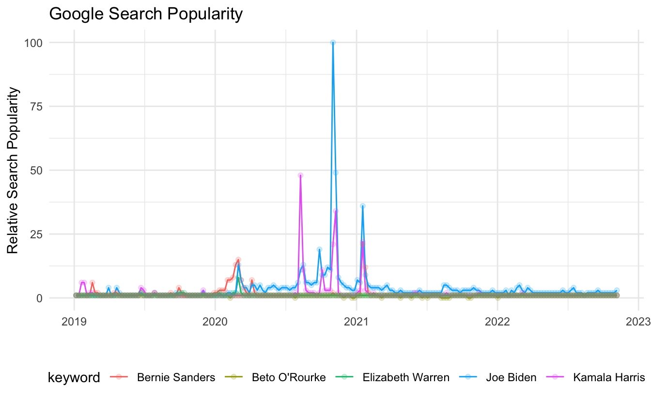
candidate_trends %>%
  get_interest() %>%
  ggplot(aes(date, hits, color = keyword)) +
  geom_line() +
  geom_point(alpha = .2) +
  theme_minimal() +
  theme(legend.position = "bottom") +
  labs(x = "",
       y = "Relative Search Popularity",
       title = "Google Search Popularity")
It is also possible to view the related search queries for a given set of keywords using get_related_queries().
candidate_trends %>%
  get_related_queries() %>%
  group_by(keyword) %>%
  sample_n(2)
#> # A tibble: 10 × 5
#> # Groups:   keyword [5]
#>    subject  related_queries value                        keyword          category
#>    <chr>    <chr>           <chr>                        <chr>            <chr>
#>  1 +3,450%  rising          klobuchar                    Bernie Sanders   All categories
#>  2 81       top             joe biden                    Bernie Sanders   All categories
#>  3 32       top             kamala harris                Beto ORourke     All categories
#>  4 Breakout rising          beto orourke announcement    Beto ORourke     All categories
#>  5 Breakout rising          elizabeth warren beer video  Elizabeth Warren All categories
#>  6 40       top             elizabeth warren net worth   Elizabeth Warren All categories
#>  7 Breakout rising          joe biden stimulus           Joe Biden        All categories
#>  8 Breakout rising          joe biden senile             Joe Biden        All categories
#>  9 Breakout rising          kamala harris husbands       Kamala Harris    All categories
#> 10 30       top             vice president kamala harris Kamala Harris    All categories